Text + Image Essay · Windows into Consciousness
Adrian’s Neuron Revisited
From threshold and firing rate to a nested, nonlinear attractor engine
14 text sections · 14 images · 33-part flow
Adrian’s neuron — opened from within
Adrian’s four properties remain sound as phenomenology.
The modern neuron, however, is not a passive relay with one threshold and one output: it is an active nonlinear dynamical system with nested attractor layers, bifurcation-specific codes and homeostatic mechanisms that continuously reposition B2.
“Every spike is an Omega event. Every inter-spike interval is a MIR measurement. The neuron is not a wire — it is a single-unit implementation of the entire energy-information attractor framework, operating at the cellular scale.”
Four properties, one attractor system
All-or-none
Threshold is B2: below it, activity returns to rest; above it, the membrane completes a stereotyped limit-cycle orbit.
Exponential range
Logarithmic encoding lets orders of magnitude of stimulus intensity occupy a modest linear range of firing rates.
Rate coding
If spikes are identical, timing remains free: inter-spike interval carries stimulus intensity through the rhythm of the orbit.
Adaptation + inhibition
Slow potassium currents and inhibitory interneurons correct drift toward the supercritical regime at different timescales.

Adrian’s first property
All-or-none — threshold as B2
The spike threshold is B2, the neuron’s bifurcation point. Below it, activity returns to the resting fixed-point attractor; above it, the membrane completes the same stereotyped limit-cycle orbit, however far the stimulus exceeds threshold.
Spike amplitude therefore carries no information. Graded input has been compressed into a binary event: one bit per spike.

Adrian’s second property
Exponential range — criticality’s dynamic range
Across a population, logarithmic encoding lets orders of magnitude of stimulus intensity occupy a modest linear range of firing rates. In this account, that dynamic range belongs to criticality: a subcritical neuron saturates too quickly, while a supercritical one runs away.
Adrian observed the phenomenology; criticality supplies its attractor logic.
Adrian’s third property
Rate coding — the carrier is temporal
If spikes are identical, the remaining free variable is when they arrive. The inter-spike interval is the neuron’s MIR measure: the frequency with which the limit cycle is completed tells a downstream neuron about stimulus intensity.
The cell acts as a biological frequency modulator, converting amplitude into the rhythm of an attractor orbit.
Adrian’s fourth property
Adaptation and inhibition — the return
Sustained firing recruits slow potassium currents that hyperpolarise the membrane and effectively raise B2. Inhibitory interneurons detect rising local activity and suppress it through GABA.
At different timescales, both detect drift toward the supercritical regime and return the system toward critical operation: adaptation is the cell’s HSTP; inhibition is the circuit’s HSTP.

The single law underneath
One dynamical structure, read four ways
Adrian measured these properties in single sensory nerve fibres from crabs and frogs without a mathematical framework for their universality. Read together, they are one law stated four ways: a threshold bifurcation, a logarithmic attractor encoding function, a limit-cycle frequency as information carrier, and a homeostatic return mechanism.
Their common origin is a dynamical structure that compresses graded input, carries information in temporal rhythm and preserves stability near B2.
THE MODERN CORRECTION
The cellular phase space was opened
The fundamental revision is not that Adrian’s neuron was discarded, but that its cellular phase space was opened.
A pyramidal neuron can occupy different attractor states in its dendrites and soma at the same time, integrating top-down context with bottom-up sensory input through a nonlinear relation that a point-neuron model cannot express.

One cell, three nested layers
DISTAL
NMDA spikes create local plateau potentials lasting hundreds of milliseconds, independently of the soma: the first attractor layer.
PROXIMAL
Calcium spikes integrate across branches: a second layer that can amplify or veto distal input.
SOMA + AXON
Classical Hodgkin–Huxley dynamics form the third layer — the layer Adrian was measuring.
A single cell is not one attractor but a nested cascade of local attractor compartments.
Coding follows bifurcation geometry
Izhikevich’s correction: rate coding is not a universal neural language; it is the strategy of one bifurcation type.
Regular-spiking
Saddle-node dynamics encode intensity as rate.
Fast-spiking
A Hopf bifurcation resonates at preferred frequencies and encodes timing.
Bursting
A SNIC bifurcation announces salience in high-MIR packets.
Chattering
Coexisting limit cycles encode categorical distinctions.
Different regions of bifurcation space implement different Ω strategies.
Homeostasis actively reshapes B2
I_AHP · adaptation reread
The I_AHP current is not passive fatigue. Each spike deposits calcium, opens slow potassium channels and shifts the fixed-point attractor away from B2.
The neuron counts its firing history and raises its own threshold.
I_h · the complementary return
During prolonged hyperpolarisation, the I_h current activates and depolarises the cell back toward threshold.
It is the rebound attractor: the self-righting mechanism after inhibition.
Inhibitory Interneurons — a layered attractor sculptor
PV
Output gate. Targets the soma and axon initial segment, setting the effective somatic B2 with millisecond precision.
SST
Dendritic gate. Targets distal dendrites, closing access to plateau potentials without silencing the soma.
VIP
Contextual gate. Inhibits PV and SST cells, providing contextual disinhibition when access should open.
A cellular HSTP decides which compartments are accessible, in which context and at which moment.

From neuron to cognition
Coupling creates new attractor geometry
When neurons couple, their phase spaces multiply rather than merely add, allowing sustained states, oscillations and winner-take-all competitions that no isolated cell possesses.
Across synapse, dendrite, soma, column, area and global brain state, each B2 crossing generates a qualitatively new attractor while higher levels constrain lower ones through gain control.
Thinking is the trajectory; the thought is the attractor in which it settles.
Adrian’s neuron — revisited
Adrian’s four properties were correct as phenomenology but wrong as mechanism. The neuron is not a relay. It is a fractal attractor engine — nested B2 crossings, distinct Ω strategies and dedicated homeostatic returns, all within a single cell.

Six scales — six attractor geometries — six B2 crossings
Synaptic attractor — vesicle release probability defines a stochastic fixed point. LTP/LTD are B2 crossings: the synapse flips between weak and strong attractor states. Each synapse is a 1-bit memory with its own bistable attractor basin.
Dendritic attractor — NMDA plateau potentials. The branch integrates its synaptic inputs and either stays subthreshold (fixed point) or fires a local plateau (limit cycle). Branch-specific learning. First spatial attractor.
Somatic attractor — HH dynamics. Resting fixed point → action potential limit cycle. Bifurcation type (saddle-node, Hopf, SNIC) determines encoding strategy. Adaptation actively repositions B2 via I_AHP.
Column attractor — ~10,000 neurons. Sustained activity states (up-states) are strange attractors that cannot exist in a single neuron. Recurrent excitation among pyramidal cells creates winner-take-all basins. The column’s B2 crossing is the emergence of a working memory representation.
Area attractor — millions of neurons. Gamma oscillations (30–80Hz) emerge from PING circuits — not present at single-neuron level. Cross-frequency coupling: theta phase gates gamma amplitude. The area’s B2 is the transition from noise to organised oscillation — an entirely new attractor topology.
Global attractor — default mode network, salience network, executive network. Brain states (waking, REM, NREM) are macroscopic strange attractors spanning the entire organ. Consciousness is the global attractor that all lower attractors collectively inhabit. B2 crossing = ignition — the transition from local to global brain state.
Each rung is not just the rung below it scaled up. Each B2 crossing produces a qualitatively new type of attractor — sustained states, oscillations, and global ignition cannot be predicted from the dynamics at the scale below. This is the formal definition of emergence: new attractor geometry appearing at each B2 crossing that is irreducible to the level below.
What a Hamiltonian system is
A Hamiltonian system is any physical system fully described by a single scalar function H — the Hamiltonian — which equals the system’s total energy. The equations of motion fall out of H automatically. No energy is added or lost: total energy is conserved. The system evolves through phase space, trading energy between kinetic and potential forms but never gaining or losing it overall.
q — generalised positions
Where each particle is in configuration space. Could be spatial coordinates, angles, membrane voltage — any degree of freedom.
p — generalised momenta
The conjugate momentum to each position. Together (q, p) define a point in phase space — the complete state of the system.
Phase space — where everything happens
Phase space is the 2N-dimensional space of all possible (q, p) pairs for an N-particle system. The system’s entire history is a single trajectory through this space. Crucially: phase space volume is conserved — Liouville’s theorem. The trajectory cannot contract to a point or expand to fill everything. This is what distinguishes Hamiltonian systems from dissipative ones.
Integrable regime
Trajectories lie on smooth N-dimensional tori in phase space. Regular, predictable, periodic. Zero KS entropy. Ω → 0.
Chaotic regime
Tori break down. Trajectories wander through a chaotic sea — bounded but never repeating. Positive KS entropy. Strange attractor. Ω ≫ 1.
Mixed regime
KAM theorem: tori and chaotic regions coexist. Islands of regularity embedded in a chaotic sea. Most real systems live here.
Everything in one table
| Concept | Hamiltonian meaning | Neural meaning | Ω reading |
|---|---|---|---|
| H | total energy = KE + PE | metabolic energy = ATP | the engine |
| phase space | (q,p) for all particles | all neural states | where attractors live |
| λ₁ | trajectory divergence rate | sensitivity to input | determines MIR ceiling |
| h_KS | information production rate | EEG complexity | = Σλᵢ (positive) |
| MIR | KE↔PE correlation rate | inter-region synchrony | ≤ h_KS |
| β | power-law exponent | nonlinearity of brain | determines Ω scaling |
| Ω | Ė/MIR = (MIR)^(β−1) | info per metabolic joule | order parameter |
| B₂ | bifurcation to chaos | criticality threshold | emergence point |
| attractor | phase space subset | brain/cognitive state | where Ω is sustained |
| S | thermodynamic entropy | metabolic heat | ≥ k_B · h_KS |
Adrian’s neuron vs the modern attractor neuron
Adrian 1926 — point neuron
- Passive dendrites — just summate inputs
- Single threshold at soma
- Spike = binary output, no internal structure
- Rate = stimulus intensity, linearly
- Neuron is a relay — input → output
- Adaptation = fatigue, passive decay
Modern — dynamical attractor neuron
- Active dendrites — compute, not just sum
- Multiple bifurcation points across compartments
- Spike = attractor transition, rich internal dynamics
- Rate = one of many coding schemes
- Neuron is a dynamical system — computes attractors
- Adaptation = active homeostatic attractor drift
Foundation — Hodgkin-Huxley (1952) reread as attractor dynamics
The action potential is a limit-cycle orbit in a 4D phase space
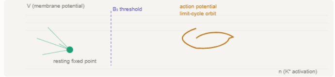
Hodgkin & Huxley’s equations — V, m, h, n — define a 4-dimensional dynamical system. The resting state is a stable fixed-point attractor. The action potential is not a passive discharge — it is a transient excursion along a limit-cycle orbit, driven by the bifurcation structure of sodium and potassium conductances. Adrian’s all-or-none law is the binary nature of this bifurcation.
Resting state — stable fixed point
V = −70mV is a globally attracting fixed point. Na⁺ channels closed. K⁺ channels maintain hyperpolarisation. All perturbations below threshold return here exponentially — a true attractor basin.
Spike — limit cycle orbit
Above threshold, Na⁺ channels undergo a saddle-node bifurcation — the fixed point loses stability and the trajectory is captured by a limit-cycle orbit. The spike shape is the orbit geometry. Identical spikes = identical orbits.
Key mechanism — cross-frequency coupling as inter-scale B₂ gating
Theta gates gamma — the brain’s inter-scale attractor communication protocol
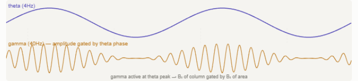
The most concrete example of inter-scale attractor interplay is cross-frequency coupling (CFC). Theta oscillations (4–8Hz) at the area scale phase-modulate gamma oscillations (30–80Hz) at the column scale — gamma amplitude is highest at the peak of theta phase. This is one attractor (theta) gating the B2 crossing of another (gamma onset).
Theta — hippocampal attractor
4–8Hz oscillation. Encodes spatial and temporal context. Its phase defines windows of excitability — when the network is near its B2 and when it is far from it.
Gamma — column attractor
30–80Hz oscillation from PING circuits. Encodes specific content — which neurons fire within the gamma cycle encodes feature identity. Only possible when theta says the moment is important.
Coupling = Ω transfer
The theta-gamma coupling is the inter-scale MIR: information about context (theta) modulates information about content (gamma). The Ω of the column depends on the phase of the area attractor.

The interplay — how scales create each other
Bottom-up emergence and top-down constraint — the two directions of attractor coupling
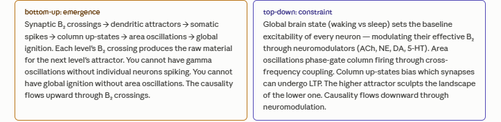
The fractal hierarchy is not one-directional. Lower scales create higher-scale attractors through emergence. Higher-scale attractors constrain lower-scale dynamics through top-down modulation. Both directions operate simultaneously — the brain is a bidirectional attractor hierarchy.
Bottom-up: emergence
Synaptic B2 crossings → dendritic attractors → somatic spikes → column up-states → area oscillations → global ignition. Each level’s B2 crossing produces the raw material for the next level’s attractor.
Top-down: constraint
Global brain state sets the baseline excitability of every neuron — modulating their effective B2 through neuromodulators. Area oscillations phase-gate column firing through cross-frequency coupling. Column up-states bias which synapses can undergo LTP.

Basin transitions — cognition as attractor navigation
Every cognitive act is a trajectory through nested attractor basins
Perception, memory, decision, action — each is a specific sequence of B2 crossings propagating up and down the fractal hierarchy simultaneously.
- sensory input
- synaptic B₂
- dendritic plateau
- somatic spike
- column up-state
- gamma burst
- global ignition
- perception
- top-down prediction
- neuromodulator release
- area B₂ shift
- column B₂ shift
- synaptic gain change
- attention
Modern revision 1 — active dendrites as distributed attractor landscape
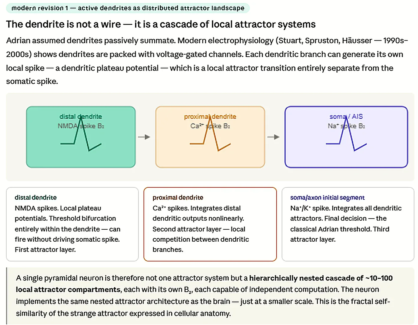
The dendrite is not a wire — it is a cascade of local attractor systems
Adrian assumed dendrites passively summate. Modern electrophysiology shows dendrites are packed with voltage-gated channels. Each dendritic branch can generate its own local spike — a dendritic plateau potential — which is a local attractor transition entirely separate from the somatic spike.
DISTAL dendrite
NMDA spikes. Local plateau potentials. Threshold bifurcation entirely within the dendrite — can fire without driving somatic spike. First attractor layer.
PROXIMAL dendrite
Ca²⁺ spikes. Integrates distal dendritic outputs nonlinearly. Second attractor layer — local competition between dendritic branches.
SOMA + AXON initial segment
Na⁺/K⁺ spike. Integrates all dendritic attractors. Final decision — the classical Adrian threshold. Third attractor layer.
A single pyramidal neuron is therefore not one attractor system but a hierarchically nested cascade of ~10–100 local attractor compartments, each with its own B2, each capable of independent computation. The neuron implements the same nested attractor architecture as the brain — just at a smaller scale.
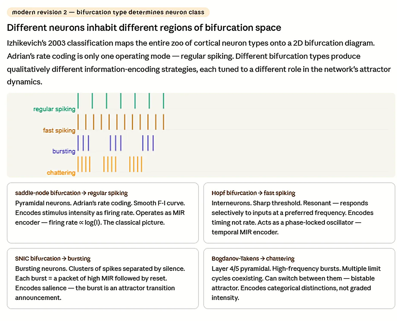
Modern revision 2 — bifurcation type determines neuron class
Different neurons inhabit different regions of bifurcation space
Izhikevich’s 2003 classification maps the entire zoo of cortical neuron types onto a 2D bifurcation diagram. Adrian’s rate coding is only one operating mode — regular spiking. Different bifurcation types produce qualitatively different information-encoding strategies, each tuned to a different role in the network’s attractor dynamics.
Saddle-node bifurcation → regular spiking
Pyramidal neurons. Adrian’s rate coding. Smooth F-I curve. Encodes stimulus intensity as firing rate. Operates as MIR encoder — firing rate ∝ log(I). The classical picture.
Hopf bifurcation → fast spiking
Interneurons. Sharp threshold. Resonant — responds selectively to inputs at a preferred frequency. Encodes timing not rate. Acts as a phase-locked oscillator — temporal MIR encoder.
SNIC bifurcation → bursting
Bursting neurons. Clusters of spikes separated by silence. Each burst = a packet of high MIR followed by reset. Encodes salience — the burst is an attractor transition announcement.
Bogdanov-Takens → chattering
Layer 4/5 pyramidal. High-frequency bursts. Multiple limit cycles coexisting. Can switch between them — bistable attractor. Encodes categorical distinctions, not graded intensity.
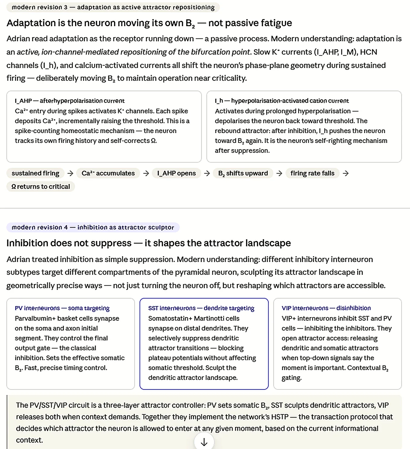
Modern revision 3 — adaptation as active attractor repositioning
Adaptation is the neuron moving its own B2 — not passive fatigue
Adrian read adaptation as the receptor running down — a passive process. Modern understanding: adaptation is an active, ion-channel-mediated repositioning of the bifurcation point. Slow K⁺ currents (I_AHP, I_M), HCN channels (I_h), and calcium-activated currents all shift the neuron’s phase-plane geometry during sustained firing — deliberately moving B2 to maintain operation near criticality.
I_AHP — afterhyperpolarisation current
Ca²⁺ entry during spikes activates K⁺ channels. Each spike deposits Ca²⁺, incrementally raising the threshold. This is a spike-counting homeostatic mechanism — the neuron tracks its own firing history and self-corrects Ω.
I_h — hyperpolarisation-activated cation current
Activates during prolonged hyperpolarisation — depolarises the neuron back toward threshold. The rebound attractor: after inhibition, I_h pushes the neuron toward B2 again. It is the neuron’s self-righting mechanism after suppression.
Modern revision 4 — inhibition as attractor sculptor
Inhibition does not suppress — it shapes the attractor landscape
Adrian treated inhibition as simple suppression. Modern understanding: different inhibitory interneuron subtypes target different compartments of the pyramidal neuron, sculpting its attractor landscape in geometrically precise ways — not just turning the neuron off, but reshaping which attractors are accessible.
PV interneurons — soma targeting
Parvalbumin+ basket cells synapse on the soma and axon initial segment. They control the final output gate — the classical inhibition. Sets the effective somatic B2. Fast, precise timing control.
SST interneurons — dendrite targeting
Somatostatin+ Martinotti cells synapse on distal dendrites. They selectively suppress dendritic attractor transitions — blocking plateau potentials without affecting somatic threshold.
VIP interneurons — disinhibition
VIP+ interneurons inhibit SST and PV cells — inhibiting the inhibitors. They open attractor access: releasing dendritic and somatic attractors when top-down signals say the moment is important.
The PV/SST/VIP circuit is a three-layer attractor controller: PV sets somatic B2, SST sculpts dendritic attractors, VIP releases both when context demands. Together they implement the network’s HSTP — the transaction protocol that decides which attractor the neuron is allowed to enter at any given moment, based on the current informational context.